Sharpe 1.9 | Why Overnight Moves Reverse During the Day

Premise

Most people calculate a “daily return” simply using yesterday’s close to today’s close (close→close). However that single number hides what happens inside the day.

If we split the day into two return segments, the overnight return (close→open) and the intraday return (open→close), we can ask a simple question: do these returns behave the same, or differently and do they have any predictability?

Our plan is deliberately plain: Let’s create a set of different price returns (close→open, open→open, close→close etc.) from end-of-day price data and see if we can find an edge in the data.

As with every strategy we investigate, we look at the evidence first and the strategy second.

Idea

There’s a growing body of research showing that very short-horizon returns can predict future returns. One of the oldest examples is the reversal strategy: yesterday’s close→close return helps forecast tomorrow’s return, that is, big winners tend to cool off, big losers tend to bounce. But this strategy over recent times has tended to lose it’s edge and s the alpha is no longer tradeable.

We’re going to take that idea and sharpen it. Instead of treating the day as one block, we decompose the close-to-close return into two pieces, the overnight return (close→open, CO) and the intraday return (open→close, OC). We can now ask a tighter question:

Can overnight returns reliably signal a reversal in the intraday return?

So in this article we take a look at overnight–intraday mean-reversion, denoted CO-OC. In plain terms, we buy assets with low past overnight returns and sell assets with high past overnight returns, then hold those positions during the next intraday session. If overnight moves overshoot, the day session should mean-revert them — and that’s the edge we’re testing.

The Edge

We test this idea across a broad set of equity sectors and equity index futures. Instead of testing the CO-OC strategy in isolation, we create various different strategies to test along with the CO-OC strategy.

We keep the Notation nice and simple. Each strategy we test is written as AB–CD:

• AB = the formation window we use to build the signal.
• CD = the holding window where we take risk and realise P&L.

Each strategy is defined below:

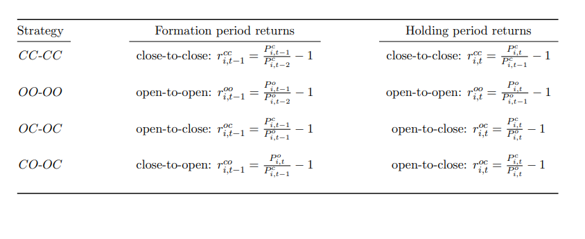
From formation returns to a market-neutral portfolio

1. For each day, we compute the formation returns across the universe and demean them cross-sectionally.
2. Demeaning has a great property: the signals sum to zero.
   If we map signal → weight linearly, the weights also sum to zero.
3. Result: an equal-weight long/short, market-neutral portfolio with very low market risk by construction.
4. We then double the weight of each asset, so we invest 100% of the Portfolio Value in long and -100% short, keeping us market neutral.

We Winsorize the returns two-sided to keep outliers from dominating, then evaluate summary statistics, t-stats and annualized Sharpe for each setup.

Strategy Stats: Equity Futures

Below are the results for the various strategies we are testing using Equity Futures (ES, YM, NQ, EMD, NKD and RTY):

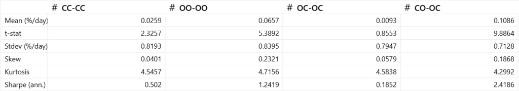
From the above we can see that, while the standard close-to-close and open-to-open strategies show some signal, the CO–OC strategy dominates. It delivers the highest daily returns, the strongest statistical significance, and by far the best risk-adjusted performance.

Strategy Stats: Equity Biotech Sector ETF’s

Below are the results for the strategies using Equity Biotech ETF’s (ARKG, XBI and IBB):

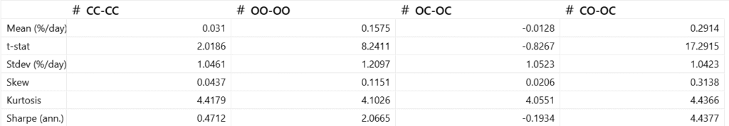
Across the four reversal strategies, the CO–OC strategy stands out again with the strongest performance: an average daily return of ~0.29%, a very high t-stat (17.3), and an annualised Sharpe ratio of 4.44. Overall, the evidence confirms that the overnight-to-intraday reversal (CO–OC) captures the most robust and statistically significant mean-reversion effect.

Strategy Stats: Equity Financials Sector ETF’s

Below are the results for the strategies using Equity Financials ETF’s ( IYF, XLF, VFH, FNCL):

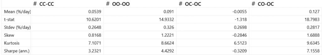
When applied to financial ETFs, all four reversal strategies show clear differences in performance. The CO–OC strategy once again dominates, delivering an average daily return of ~0.13%, an extremely high t-stat (18.8), and an annualised Sharpe ratio above 9.0 — making it the strongest and most reliable signal.

At this point, the evidence is clear, across broad markets, the CO–OC strategy consistently delivers the strongest short-term reversal effect. It outperforms alternative formulations on both return and risk-adjusted bases, with Sharpe ratios that are multiple times higher than the others.

With the edge firmly established, the next natural step is to see how the strategy performs when traded. In other words, if we actually put capital behind this signal, entering at the open and exiting at the close, what kind of return profile, drawdowns, and consistency should we expect?

The CO–OC strategy consistently delivers the strongest short-term reversal effect.

The Strategy

Below we run the CO–OC short-term reversal strategy in our back-tester across three different universes and also consider commissions:

1. US Equity Futures
2. US Biotech Sector ETFs
3. US Financials Sector ETFs

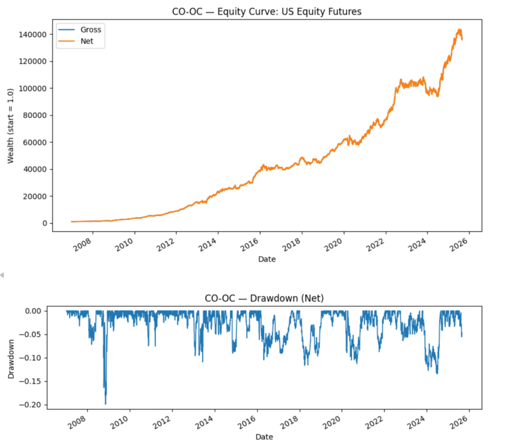
US Equity Futures

Below is the backtest CO-OC strategy on the equity futures universe:

Metric	Value
Start Date	2007-01-01
End Date	2025-09-01
Start Capital	$1,000.0
End Capital	$136,915.79
CAGR (net)	30.31%
Annualized Stdev (net)	13.01%
Net Sharpe (ann.)	2.09
Max Drawdown (net)	-19.93%

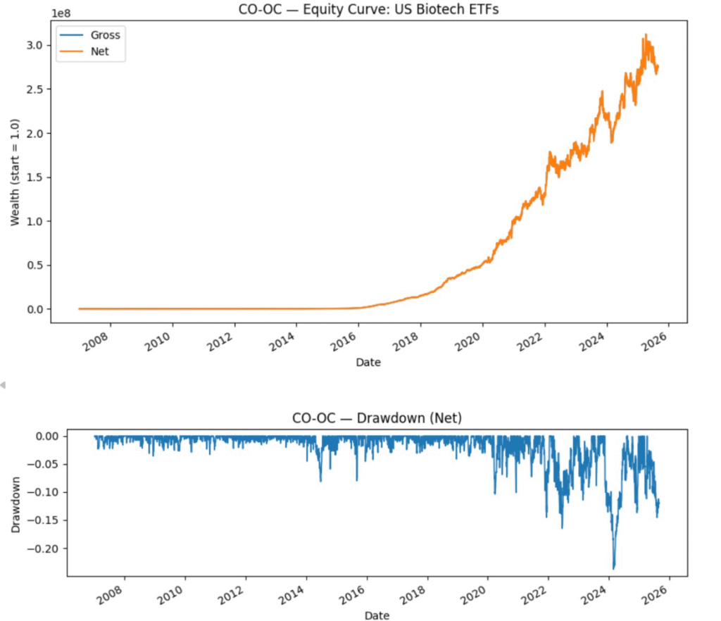
US Biotech Sector ETFs

Below is the backtest CO-OC strategy on the US Biotech Sector ETF universe:

Metric	Value
Start Date	2007-01-01
End Date	2025-09-01
Start Capital	$1,000.00
End Capital	$274,858,131.11
CAGR (net)	95.69%
Annualized Stdev (net)	17.60%
Net Sharpe (ann.)	3.91
Max Drawdown (net)	-23.80%

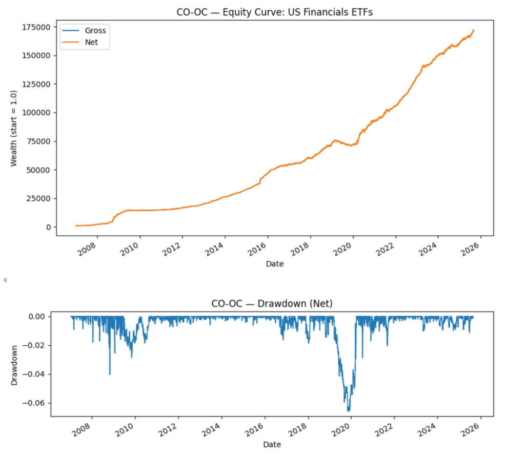
US Financials Sector ETFs

Below is the backtest CO-OC strategy on the US Financials Sector ETF universe:

Metric	Value
Start Date	2007-01-01
End Date	2025-09-01
Start Capital	$1,000.00
End Capital	$171,945.47
CAGR (net)	31.79%
Annualized Stdev (net)	7.62%
Net Sharpe (ann.)	3.67
Max Drawdown (net)	-6.60%

Practical caveat

A key challenge with this strategy is that both the signal and the execution depend on the opening price. To implement it correctly, you need to know the precise open in order to size trades — but you also need to trade at that very same open. For retail investors, this is extremely difficult because access to indicative opening prices is limited.

This makes the CO–OC reversal strategy better suited to professional or well-capitalised investors who can access exchange auction data and submit trades into the opening auction with confidence of hitting the Open price.

Conclusion

The CO-OC short-term reversal strategy demonstrates that overnight returns (close-to-open) contain strong predictive power for the following intraday session (open-to-close). By systematically shorting assets with high overnight gains and going long those with large overnight losses, the strategy captures mean-reversion dynamics in equity markets.

Backtests over 2007–2025 show:

• High CAGR and Sharpe ratios — indicating both strong growth and efficient risk-adjusted returns.
• Low volatility and drawdowns — suggesting robustness even during crisis periods.
• Consistent edge across sectors and futures — not limited to a single market environment.

Overall, CO-OC appears to be one of the most robust and tradable short-term reversal strategies documented in academic literature, with performance that persists across time, markets, and data samples. While implementation costs, slippage, and liquidity constraints must always be considered, the empirical evidence suggests the strategy offers a genuine repeatable edge.

Want to see how this strategy plays out in real time and the daily strategy holdings? Head over to the QuantReturns.com strategy library, where we track the strategy’s daily performance. All performance tracking is for research purposes only and does not constitute investment advice.

Disclaimer

This website provides an assessment of the market and economic environment at a specific point in time. It is not intended as a forecast of future events or a guarantee of future results. The content is meant to present ideas for further research and analysis and should not be interpreted as a recommendation to invest.

This material does not provide individualized advice or recommendations for any specific reader. Forward-looking statements are subject to risks and uncertainties, and not all relevant risks related to the ideas presented may be covered. Actual results, performance, or achievements may differ materially from those expressed or implied.

The information is based on data gathered from sources we believe to be reliable. However, its accuracy is not guaranteed, it does not purport to be complete, and it should not be used as a primary basis for investment decisions.

Readers are encouraged to conduct their own due diligence and consider their individual investment objectives, risk tolerance, time horizon, tax situation, liquidity needs, and portfolio concentration. Consulting with a professional adviser is recommended to determine whether the ideas presented here are suitable for your unique circumstances.

By using the information in this article, you agree that the author and publisher are not liable for any direct or indirect losses resulting from your use of the material.